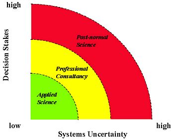
Previous: Climate Impacts

Post-Normal Science

We must think of climate change in terms of risk, not certainty.

As should be abundantly clear by now, when assessing climate science, impacts and now policy issues, we are rarely talking about certainties, but rather about risks. The climate problem, like the ozone problem (see, e.g., the EPA ozone website or the NOAA ozone website) and, in fact, almost all interesting socio-technical problems, is filled with “deep uncertainties,” uncertainties in both probabilities and consequences that are not resolved today and may not be resolved to a high degree of confidence before we have to make decisions regarding how to deal with their implications. They often involve very strong and opposite stakeholder interests and high stakes. In fact, sociologists Funtowicz and Ravetz (see, for example: Funtowicz and Ravetz, 1993) have called such problems examples of “post-normal science.” In Kuhn’s “normal science” (Kuhn, 1962), we scientists go to our labs and we do our usual measurements, calculate our usual statistics, build our usual models, and we proceed on a particular well-established paradigm. Post-normal science, on the other hand, acknowledges that while we’re doing our normal science, some groups want or need to know the answers well before normal science has resolved the deep inherent uncertainties surrounding the problem at hand. Such groups have a stake in the outcome and want some way of dealing with the vast array of uncertainties, which, by the way, are not all equal in the degree of confidence they carry. Compared to applied science and professional consultancy, post-normal science carries both higher decision stakes and higher systems uncertainty, as depicted in the graphic below, which accompanies Jerry Ravetz's website's discussion of post-normal science.

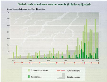
The climate change debate — particularly its policy components — falls clearly into the post-normal science characterization and will likely remain there for decades, which is the minimum amount of time it will take to resolve some of the larger remaining uncertainties surrounding it, like climate sensitivity levels and the likelihood of abrupt nonlinear events, including a possible shutoff of the Gulf Stream in the high North Atlantic (see What is the Probability of “Dangerous” Climate Change?).

And the climate problem emerges not simply as a post-normal science research issue, but as a risk management policy debate as well. Risk is classically defined as probability times consequences. One needs both. The descriptive science — what we like to call our “objective” purview — entails using empirical and theoretical methods to come up with the two factors that go into risk assessment: a) what can happen? and b) what are the odds? And both are essential. However, it’s not as simple as it sounds, as we can't possibly obtain empirical data about future climate change before the fact. Our empirical data is only about the present and the past, and therefore, the best way we can simulate the future is by constructing a systems theory — built, of course, by aggregating empirically derived sub-models. However, the full integrated systems model is not directly verifiable before the fact (i.e. until the future rolls around and proves it right or wrong — or, more likely, a mixture of both), and thus only subjective methods are available. The degree of confidence we may assign to any assessed risk is always subjective, since probabilities about future events necessarily carry some subjectivity. That doesn’t mean it is not an expert-driven assessment, but it is still subjective. So, the big question we’re left with is: what probabilities should we use and from whom do we obtain them?

There are also normative judgments, or value judgments, that must be made when considering climate change policy: what is safe and what is dangerous? The 1992 UNFCCC, which was signed by President Bush Senior (and ratified by Congress) and the leaders of about 170 other countries, essentially stated that it is the job of the Framework Convention to prevent (and this is a direct quote) “dangerous anthropogenic interference with the climate system” — although nobody knows what that means! “Dangerous” is a value judgment that depends upon the assessment of the probabilities and consequences just discussed. We scientists can provide a range of scenarios and even assign subjective likelihoods and confidence levels to them, but it’s up to policymakers to decide what risks are acceptable, and which are dangerous and should be avoided — and what course of action should be taken or not taken either way.

The other major question in the climate change debate is: what is fair? If a cost-benefit analysis is performed to find the least expensive way to achieve maximum climate abatement, it may be that in the “one dollar, one vote” world that cost-benefit methods typically imply, some action — passive adaptation, for example — might appear to be the most cost-effective. But here’s the dilemma: a rich country that has historically produced large emissions of greenhouse gases could well find it cheaper to adapt by building seawalls, for example, than to mitigate through an action such as retiring a few coal-burning power plants. On the other hand, a poorer country in the hotter equatorial area with fewer resources (and thus less adaptive capacity) might be both more harmed by climate change and less able to pay for or otherwise deal with the damages it causes because the country lacks the same degree of adaptive capacity as the richer country.  Thus, adaptation might seem cheaper in a cost-benefit analysis that aggregates all costs and benefits into equivalent dollars since the rich country, with a much larger share of world GDP, will be able to adapt more easily. But, that policy may not be fair in its distribution across rich and poor countries, which is the concept behind distributive justice/equity. Efficiency versus equity dilemmas, as just outlined, can lead to alternative political views of what should be done, and are also connected to the question of who should pay to abate risks. These equity/efficiency trade-offs are inherent in the ozone problem as well; they’re just multiplied by a much larger factor in dealing with climate change.

Go to top

Uncertainties in Climate Change Projections and Impacts

(See also Climate Science and Climate Impacts)

It is almost tautological to note that unexpected global changes, such as the development of the hole in the ozone layer, are inherently difficult to predict. It is perhaps equally non-informative to suggest that other climate “surprises” can arise in the future. But despite the difficulty prevalent in forecasting climate change and its consequences, it is imperative that we address the uncertainties underlying our understanding of climate change and its effects. Global change science and policymaking will have to deal with uncertainty and surprise for the foreseeable future. Thus, more systematic analyses of surprise issues and more formal and consistent methods of incorporation of uncertainty into global change assessments will become increasingly necessary, as exemplified in the Climate Science and Climate Impacts sections of this website (see especially What is the Probability of “Dangerous” Climate Change?).

Significant uncertainties plague projections of climate change and its consequences, but one thing is known for certain: the extent to which humans have influenced the environment since the Victorian Industrial Revolution is unprecedented. Human-induced climate change is projected to occur at a very rapid rate; natural habitats will become more fragmented as land is cleared for agriculture, settlements, and other development activities; “exotic” species are and will continue to be imported across natural biogeographic barriers; and we will persist in assaulting our environment with a host of chemical agents. For these reasons, it is essential to understand not only how much climate change is likely to occur, but also how to estimate climate damages (see Climate Impacts). Speculation on how the biosphere will respond to human-induced climate change is fraught with deep uncertainty (see Root and Schneider, 2002), but as research continues we will continue to narrow our range of plausible projections.

The combination of increasing global population and increasing energy consumption per capita is expected to contribute to increasing CO₂ and sulfate emissions over the next century. However, projections of the extent and effect of the increases are, as you might have guessed by now, very uncertain. Midrange estimates of emissions suggest a doubling of current equivalent CO₂ concentrations in the atmosphere by the middle of the 21^st century, leading to projected warming ranging from more than one degree Celsius all the way up to six degrees Celsius by the end of the twenty-first century (see Earth's surface temperature). Warming at the upper end of this range is even more likely if CO₂ concentrations reach triple or more their current levels, which could occur during the 22^nd century in about half the SRES scenarios (see CO2 concentrations). While warming at the low end of this range could still have significant implications for species adaptation, warming of five degrees or more could have catastrophic effects on natural and human ecosystems, including serious coastal flooding, collapse of thermohaline circulation (THC) in the Atlantic Ocean, and nonlinear ecosystem responses (see Reasons for climate impact concerns). The overall cost of these impacts on “market sectors” of the economy could easily run from tens of billions of dollars annually in the near term up to perhaps as much as trillions of dollars by the late 21^st century (see Probability distributions (f(x)) of climate damages), and non-market impacts (i.e., loss of human lives, loss of biodiversity — see the Five Numeraires) could be even greater.

Go to top

Decision-Making Under Uncertainty

Debate about the level of certainty required to reach a “firm” conclusion and make a decision is a perennial issue in science and policymaking. The difficulties of explaining uncertainty have become increasingly salient as politicians seek scientific advice and societies seek political advice on dealing with global environmental change. Policymakers struggle with the need to make decisions that will have far-reaching and often irreversible effects on both environment and society — against a backdrop of sparse and imprecise information. Not surprisingly, uncertainty often enters the decision-making process through catch-phrases like "the precautionary principle," "adaptive environmental management," "the preventative paradigm," or "principles of stewardship." While a preventive approach is preferable, in my view, it entails a step that many governments have been unwilling to make thus far. But in The Climate Change Challenge, Grubb, 2004 reminds us: "No business or government expects to take decisions knowing everything for certain, and climate change embodies the same dilemmas on a global and long term scale. Policymaking nearly always requires judgment in the fact of uncertainty and climate change is no different. Taking no action is itself a decision." Any shift towards prevention in environmental policy “implies an acceptance of the inherent limitations of the anticipatory knowledge on which decisions about environmental [problems] are based” (Wynne, 1992). In order for such a shift to occur, we must ask two major questions. First, how can scientists improve their characterization of uncertainties so that areas of slight disagreement do not become equated with major scientific disputes, which occurs all too often in media and political debates? (See “Mediarology”.) Second, how can policymakers synthesize this information and formulate policy based on it?

In dealing with uncertainty in the science and policy arenas, two options are typically available: 1) bound the uncertainty, or 2) reduce the effects of uncertainty. The first option involves reducing the uncertainty through data collection, research, modeling, simulation techniques, and so forth, which is characteristic of normal scientific study. However, the daunting magnitude of the uncertainty surrounding global environmental change, as well as the need to make decisions before the uncertainty is resolved, make the first option a goal that is rarely achieved. That leaves policymakers with the second alternative: to manage uncertainty rather than master it. This typically consists of integrating uncertainty directly into the policymaking process. The emphasis on managing uncertainty rather than mastering it can be traced to work on resilience in ecology, most notably by Holling (1973, 1986). Resilience refers to the ability of a system to recover from a disturbance, without compromising its overall health.

The fields of mathematics, statistics, and, more recently, physics, have all independently and concurrently developed methods to deal with uncertainty. Collectively, these methods offer many powerful means and techniques climatologists can use to conceptualize, quantify, and manage uncertainty, including frequentist probability distributions, subjective probability, and Bayesian statistical analysis, and even a method for quantifying ignorance. In addition, fuzzy set logic offers an alternative to classical set theory for situations in which the definitions of set membership are vague, ambiguous, or non-exclusive. More recently, researchers have proposed chaos theory and complexification theory in attempts to create models and theories that expect the unexpected (see the discussion and references in Schneider, Turner and Morehouse Gariga, 1998, from which much of this section has been derived). More work must be done to assure that these methods, especially subjective probability and Bayesian statistical analysis, are widely accepted and used in climate change modeling.

Scaling in Integrated Assessment Models (IAMs) of Climate Change

Strictly speaking, a surprise is an unanticipated outcome. Potential climate change, and more broadly, global environmental change, is replete with this kind of truly unexpected surprise because of the enormous complexities of the processes and interrelationships involved (such as coupled ocean, atmosphere and terrestrial systems) and our insufficient understanding of them (see, for example, Climate Surprises and a Wavering Gulf Stream?). In the IPCC SAR (IPCC 1996a), “surprises” are defined as rapid, nonlinear responses of the climatic system to anthropogenic forcing, such as the collapse of the “conveyor belt” circulation in the North Atlantic Ocean (Rahmstorf, 2000) or rapid deglaciation of polar ice sheets. Unfortunately, most climate change assessments rarely consider low-probability, high-consequence extreme events. Instead, they consider several scenarios thought to “bracket the uncertainty” rather than to explicitly integrate unlikely surprise events from the tails of the distribution associated with the assessment. Structural changes in political or economic systems and regime shifts, such as a change in public consciousness regarding environmental issues, are not even considered in most scenarios.

Integrated assessments of global change disturbances involve “end-to-end” analyses of relationships and data from the physical, biological and social sciences (e.g., see the reviews and references in Weyant et al. (1996), Morgan and Dowlatabadi (1996), Rotmans and van Asselt (1996), Parson (1996), Rothman and Robinson (1997), and Schneider (1997b). Often, data or processes are collected or simulated across vastly different scales — for example, consumption at national scales and consumer preferences at family scales, or species competition at a field plot the size of a tennis court and species range boundaries at a scale of half a continent, or thunderstorms in ten-kilometer squares and grid cells of a global climate model in squares hundreds of kilometers in length, or the response of a plant in a meter-square chamber to increased concentrations of CO₂ and the response of an ecosystem to CO₂ at biome scales of thousands of kilometers. Not only must individual disciplines concerned with the impacts of global change disturbances — like altered atmospheric composition or land use and land cover changes — often deal with orders of magnitude of difference in spatial scales, but integrated studies must bridge scale gaps across disciplinary boundaries as well (see, e.g., Root and Schneider, 2003, from which much of this discussion is adapted). For instance, how can a conservation biologist interested in the impacts of climate change on a mountaintop-restricted species scale down climate change projections from a climate model whose smallest resolved element is a grid square that is 250 kilometers on a side? Or, how can a climate modeler scale up knowledge of evapotranspiration through the sub-millimeter-sized stomata of forest leaves into the hydrological cycle of the climate model, which is resolved at hundreds of kilometers? The former problem is known as downscaling (see, e.g. Easterling et al., 2001), and the latter, up-scaling (see, e.g. Harvey, 2000b). This cross-disciplinary aspect can be particularly daunting when different scales are inherent in different sub-disciplines. Scaling problems are particularly likely when the boundary between natural and social science is crossed. Only a greater understanding of the methods and traditions of each of these sub-disciplines by practitioners in the others will help to facilitate boundary-bridging across very different disciplines operating at very different scales.

Scaling in Natural Science Forecast Models. First, let us consider natural scientific scale bridging. For a forecasting model to be credible, it must analytically solve a validated, process-based set of equations accounting for the interacting phenomena of interest. The classical reductionist philosophy in science is a belief that laws (i.e., the laws of physics) apply to phenomena at all scales. If such laws can be found (usually at small scales), then the solution of the equations that represent such laws will provide reliable forecasts at all scales. This assumes, of course, that those laws are applicable to all of the phenomena incorporated into the model.

The philosophy behind most climatic models is that solutions to the energy, momentum, and mass conservation equations should, in principle, provide credible forecasting tools. Of course, as all climate modelers have readily admitted for decades (e.g. SMIC, 1972, and IPCC 1996a), this “first principles,” bottom-up approach suffers from a fundamental practical limitation: the coupled nonlinear equations that describe the physics of the air, seas, and ice are far too complex to be solved by any known (or foreseeable) analytic (i.e., exact) technique. Therefore, methods of approximation are applied in which the continuous differential equations (i.e., the laws upon which small-scale physical theory comfortably rest) are replaced with discrete, numerical, finite difference equations. The smallest resolved spatial element of these discrete models is known as a grid cell. Because the grid cells are larger than some important small-scale phenomena, such as the condensation of water vapor into clouds or the influence of a tall mountain on wind flow or the evapotranspiration from a patch of forest, “sub-grid scale” phenomena cannot be explicitly included in the model. In order to implicitly incorporate the effects of an important sub-grid scale phenomenon into a model, top-down techniques are used, in which a mix of empiricism and fine-resolution, scale-up sub-models are applied. From this, we can create a parametric representation, or “parameterization,” of the influence of sub-grid scale processes at larger scales. Determining whether it is even possible in principle to find valid parameterizations has occupied climate modelers for decades (see Climate Modeling).

In order to estimate the ecological consequences of hypothesized climate change at small scales, a researcher must first translate his/her large-scale climate change forecast to a smaller scale. For an idea of the enormity (literally!) of this task, it could involve translating climate information at a 200x200 kilometer grid scale to, perhaps, a 20x20 meter field plot — a ten-thousand-fold interpolation! Therefore, how can climatologists possibly map grid-scale projections to landscapes or even smaller areas?

At the outset, one might ask why the atmospheric component of such detailed climate models, known as general circulation models (GCMs), use such coarse horizontal resolution. This is easy to understand given the practical limitations of modern, and even foreseeable, computer hardware resources (see, e.g., Trenberth, 1992).

A 50 x 50 kilometer scale in a model falls into the range known as “the mesoscale” in meteorology. If such a resolution were applied over the entire earth, then the amount of time required for one of today's “super computers” to run a year's worth of weather data for it would be on the order of many days. (For example, to run the NCAR CCM3 at 50 km (T239) for a year, using an IBM SP3 and 64 processors, takes 20 wall-clock days. This is not running it with a full ocean model, but with fixed Sea Surface Temperature (SST) data sets. Such tests are run, e.g., at Lawrence Livermore National Laboratory; see Scientists Create Highest Resolution Global Climate Simulations,.and Simulating the Earth's Climate.) 50 kilometers is still roughly a hundred times greater than the size of a typical cloud, a thousand times greater than the typical scale of an ecological study plot, and even greater orders of magnitude larger than a dust particle on which raindrops condense. Therefore, in the foreseeable future, it is inevitable that climate change information will not be produced directly from the grid cells of climate models at the same scale that most ecological information is gathered, nor will climate models be able to accurately account for some sub-grid-scale phenomena, such as cloudiness or evapotranspiration from individual plants — let alone leaves! However, the usual scale mismatch between climate and ecological models has caused some ecologists to attempt to produce large-scale ecological studies and some climatologists to shrink the grid sizes of their climate models. Root and Schneider, 1993, have argued that both are required, as are accurate techniques for bridging the scale gaps, which, unfortunately, will exist for at least several more decades.

In order for action to be taken to avoid or correct potential risks to environment or society, it is often necessary to establish that a trend has been detected in some variable of importance - the first arrival of a spring migrant or the latitudinal extent of the sea ice boundary, for example - and that that trend can be attributed to some causal mechanism like a warming of the globe from anthropogenic greenhouse gas increases. Pure association of trends are not, by themselves, sufficient to attribute any detectable change above background noise levels to any particular cause; explanatory mechanistic models are needed in order to obtain a high confidence level about whether a particular impact can be pinned on the suspected causal agent. Root and Schneider, 1995 argued that conventional scaling paradigms — top-down associations among variables believed to be cause-and-effect and bottom-up mechanistic models run to predict associations but for which there is no large-scale data time series to confirm — are not by themselves sufficient to provide high confidence in cause-and-effect relationships embedded in integrated assessments. Rather, a cycling between top-down associations and bottom-up mechanistic models is needed. Moreover, we cannot assign high confidence to cause-and-effect claims until repeated cycles of testing in which mechanistic models predict and large-scale data “verifies” that a claim is correct. There should also be a degree of convergence in the cycling (Root and Schneider, 2003).

Modellers continue to attempt to model more regional climate change, despite the difficulties. The European Union has provided $4.2 million in funding to a project called Prudence, which is working with various models to assess climate change in Europe (see Schiermeier, 2004b and a clarification of Schiermeier's disussion of the role of the US National Assessment of the Potential Consequences of Climate Variability and Change (USNA) by MacCracken et al., 2004). Modellers in America and Canada are now seeking funding of their own to establish a similar organization. Such regional modelling is still in its early stages of development but is definitely a step in the right direction.

Strategic Cyclical Scaling. Root and Schneider, 1995 called this iterative cycling process “strategic cyclical scaling” (SCS). The motivation behind development of the SCS paradigm stemmed from the need for: (1) better explanatory capabilities for multi-scale, multi-component interlinked environmental models (e.g., climate-ecosystem interactions or behavior of adaptive agents in responding to the advent or prospect of climatic changes); (2) more reliable impact assessments and problem-solving capabilities - predictive capacity - as has been requested by the policy community; and (3) the insufficiency of both bottom-up and top-down modeling approaches by themselves.

In SCS  (see Root and Schneider, 2003), from which much of this section is derived), both macro (top-down) and micro (bottom-up) approaches are applied to address a practical problem — in our original context, the ecological consequences of global climatic change. Large-scale associations are used to focus small-scale investigations so that the valid causal mechanisms generating the large-scale relationships will be found and applied. The large-scale relationships become the systems-scale “laws” that allow climatologists or ecologists to make more credible forecasts of the consequences of global change disturbances. “Although it is well understood that correlations are no substitute for mechanistic understanding of relationships,” Levin, 1993 observed, “correlations can play an invaluable role in suggesting candidate mechanisms for (small-scale) investigation.” SCS, however, is not only intended as a two-step process, but rather a continuous cycling between large- and small-scaled studies, with each successive investigation building on previous insights from all scales. This paradigm is designed to enhance the credibility of the overall assessment process, including policy analyses, which is why it is also called “strategic.” I believe that SCS is a more scientifically viable and cost-effective means of improving the credibility of integrated assessment compared to isolated pursuit of either the scale-up or scale-down methods.

Though SCS seems to be a more well-rounded approach, it is by no means simple. The difficulty in applying SCS is knowing when the process has converged, for that requires extensive testing against some applicable data that describes important aspects of the system being modeled. When the model is asked to project the future state of the socio-environmental system,  only analogies from past data can be used for testing since there is no empirical data,. Therefore, assessing “convergence” will require judgments as well as empirical determinations, as discussed below.

Go to top

Climate Damages and the Discount Rate

Rate of forcing matters. Even the most comprehensive coupled-system models are likely to have unanticipated results when forced to change very rapidly by external disturbances like CO₂ and aerosols. Indeed, some of the transient coupled atmosphere-ocean models which are run for hundreds of years into the future exhibit dramatic change to the basic climate state (see Climate Surprises and a Wavering Gulf Stream?).

Estimating Climate Damages. A critical issue in climate change policy is costing climatic impacts, particularly when the possibility for nonlinearities, surprises, and irreversible events is allowed. The assumptions made when carrying out such estimations largely explain why different authors obtain different policy conclusions (see Dangerous Climate Impacts and the Five Numeraires).

One way to assess the costs of climate change is to evaluate the historic losses from extreme climatic events, such as floods, droughts, and hurricanes (Alexander et al., 1997). Humanity remains vulnerable to extreme weather events. Catastrophic floods and droughts are cautiously projected to increase in both frequency and intensity with a warmer climate and the influence of human activities such as urbanization, deforestation, depletion of aquifers, contamination of ground water, and poor irrigation practices (see IPCC: 1996a, 2001b, and the table Projected effects of global warming). The financial services sector has taken particular note of the potential losses from climate change. Losses from weather-related disasters in the 1990s were eight times higher than in the 1960s. Although there is no clear evidence that hurricane frequency has changed over the past few decades (or will change in the next few decades), there is overwhelming data that damages from such storms has increased astronomically (see figure below). Attribution of this trend to changes in socioeconomic factors (e.g., economic growth, population growth and other demographic changes, or increased penetration of insurance coverage) or to an increase in the occurrence or intensity of extreme weather events, as a result of global climate change, is uncertain and controversial. (Compare Vellinga et al., which acknowledges both influences and recognizes the difficulty in attribution, to Pielke Jr. and Landsea, 1998, which, in the context of hurricane damage, dismisses any effects of climate change and says increased damages result solely from richer people moving into harm’s way. However, Pielke and Downton, 2000, do suggest that for non-coastal casualty losses, climate is a partial factor — see “Population and wealth...”.)

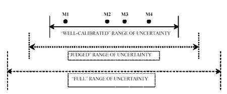
Figure — The economic losses from catastrophic weather events have risen globally 10-fold (inflation-adjusted) from the 1950s to the 1990s, much faster than can be accounted for with simple inflation. The insured portion of these losses rose from a negligible level to about 23% in the 1990s. The total losses from small, non-catastrophic weather-related events (not included here) are similar. Part of this observed upward trend in weather-related disaster losses over the past 50 years is linked to socio-economic factors (e.g., population growth, increased wealth, urbanization in vulnerable areas), and part is linked to regional climatic factors (e.g., changes in precipitation, flooding events). (Source: IPCC TAR Synthesis Report, figure 2-7.)

Many projections have been made regarding the extent of future climate-related damages. For example, Nicholls et al., 1999 project that if fossil fuel usage continues to grow at the current rate and climate changes as they expect, by 2080, the number of additional people affected by flooding in delta areas like the Nile, the Mekong, and Bangladesh and in coastline cities and villages in India, Japan, and the Philippines would be in the hundreds of millions (assuming no adaptation measures are implemented). Using four different emissions scenarios, researchers at the UK's Office of Science and Technology (OSTP) concluded that by 2080, the combination of sea level rise and increased stormy weather will likely cause storm surges to hit areas farther inland and could have the potential to increase flood risk to as much as 30 times present levels. In the worst-case scenario, serious storms that now occur only about once per century would become recurring events, coming every three years. Under this scenario, British inhabitants at risk of serious flooding would more than double to 3.5 million, and weather-related damages would skyrocket (see the UK's OSTP Foresight website, which is home to the Flood and Coastal Defense project).

An assumption in cost-benefit calculations within the standard assessment paradigm is that “nature” is either constant or irrelevant. Since “nature” falls out of the purview of the market, cost-benefit analyses typically ignore its non-market value. For example, ecological services such as pest control and waste recycling are omitted from most assessment calculations (Vellinga et al., 2001). Implicitly, this assumes that the economic value of ecological services is negligible or will remain unchanged with human disturbances. However, many authors have acknowledged that natural systems are likely to be more affected than social ones (see Root et al., 2003 and IPCC, 2001b). Recent assessments of the value of ecosystem services (e.g., Daily and Ellison, 2002) acknowledge the tremendous public good (i.e., free) provided, not to mention the recreational and aesthetic value. For example, a cost-assessment study done in New York discovered that paying residents and farmers in the Catskills to reduce toxic discharges and other environmental disruptions would provide a natural water purification service, producing savings to New York City on the order of billions of dollars relative to building new water treatment plants. Furthermore, it is highly likely that communities of species will be disrupted, especially if climate change occurs in the middle to upper range projected (Root and Schneider, 2002). These costs are rarely included in most cost-benefit calculations.

Cost-benefit analyses can be flawed in other ways, too. Phillip E. Graves, an economist at the University of Colorado at Boulder, also believes that the public-good nature of environmental goods causes difficulties in valuing them and thus in finding solutions for environmental problems. He argues that if people could pay for public goods like environmental protection in the same way that they pay for private goods -- i.e., from income -- then they would divert some of their spending from private to public goods, by making a different balance between income and leisure then they are now able to make. But since people know they can't buy public goods in the market, they don't, in this kind of CBA, devote income toward them; such miscalculation causes most economists to come up with artificially low "optimal" levels of public goods (see Graves, 2003).

The discount rate. Discounting plays a crucial role in the economics of climate change, yet it is a highly uncertain techniquer. Discounting is a method to aggregate costs and benefits over a long time horizon by summing net costs (or benefits), which have been subjected to a discount rate typically greater than zero, across future time periods. If the discount rate equals zero, then each time period is valued equally (case of infinite patience). If the discount rate is infinite, then only the current period is valued (case of extreme myopia). The discount rate chosen in assessment models is critical, since abatement costs will be typically incurred in the relatively near term, but the brunt of climate damages will be realized primarily in the long term. Thus, if the future is sufficiently discounted, present abatement costs, by construction, will outweigh discounted future climate damages. The reason is, of course, that discount rates will eventually reduce future damage costs to negligible present values.

Consider a climate impact that would cost 1 billion dollars 200 years from now. A discount rate of 5% per year would make the present value of that future cost equal to $58,000. At a discount rate of 10% per year, the present value would only be $5. Using a higher discount rate will result in more damaging effects than a lower rate. As Perrings, 2003 notes, "The effect of discounting is both to increase the potential for unexpected future costs, and to eliminate those costs from consideration." Changes in the discount rate largely explain why some authors (Nordhaus, 1994b; Nordhaus and Yang, 1996; Manne and Richels, 1997; and Nordhaus and Boyer, 2000) using large discount rates conclude that massive CO₂ emission increases are socially beneficial — i.e., more economically efficient than cuts — whereas others (Cline, 1992; Azar and Sterner, 1996; Hasselmann et al., 1997; Schultz and Kasting, 1997; Mastrandrea and Schneider, 2001; Lind, 1982) using low or zero discount rates justify substantial emission reductions, even when using similar damage functions (Portney and Weyant, 1999) ^{Note 1}. 

It would seem that the appropriate discount rate would be a matter of empirical determination, but in reality, choosing a discount rate involves a serious normative debate about how to value the welfare of future generations relative to current ones. Moreover, it requires that this generation estimate what kinds of goods and services future generations will value — e.g., how they will want to make trade-offs between material wealth and environmental services. 

There are two basic methods for deciding on a discount rate. The descriptive approach chooses a discount rate based on observed market interest rates in order to ensure that investments are made in the most profitable projects. Supporters of this approach often argue that using a market-based discount rate is the most efficient way to allocate scarce resources used for competing priorities, one of which is mitigating the effects of climate change.

The prescriptive approach emphasizes that the choice of discount rate entails a judgment about how the future should be valued. Proponents of intergenerational equity often argue that it is difficult to find an argument supporting the discounting of the welfare of future generations. Why should future people count less just because they don't exist today?

Although these two approaches are the most commonly used to pick discount rates for use in IAMs of climate change, alternative discount methods have been proposed (see Schneider and Kuntz-Duriseti, 2002, from which much of this section has been derived — further references can be obtained from that chapter). There is empirical evidence to suggest that individuals exhibit “hyperbolic discounting”, where discount rates decline over time, with higher-than-market discount rates in the short run and lower-than-market discount rates over the long term (Ainslie, 1991). This behavior is consistent with a common finding that “human response to a change in a stimulus is inversely proportional to the preexisting stimulus” (Heal, 1997). Hyperbolic discounting can be derived from both the descriptive and the prescriptive approach and is obtained when discount rates fall over time. This can be modeled in IAMs with a logarithmic discount factor or by assuming that per capita income grows logistically (i.e., diminishes over time) over the next century; since the discount rate is proportional to growth rates, declining discount rates are obtained. (See the strong case made for declining discount rates in Weitzman, 2001.)

Furthermore, if climate change is extremely severe, such that future income falls rather than grows (the latter is assumed in almost all IAMs), then the discount rate could be negative, provided that the rate of time preference is sufficiently low (Azar and Johansson, 1996). In this case, future welfare should be valued more than the present. (For a definition of rate of time preference, see the latter part of the discussion on Climate Surprises in What is the Probability of “Dangerous” Climate Change?.)

Agency. The predominant approach to the discounting problem is based on an infinitely-lived representative agent (ILA) who maximizes utility from a future welfare stream subject to economic and environmental conditions, usually assumed to be known. The representative agent framework imposes strong assumptions regarding intergenerational fairness (Solow, 1974a; and Solow, 1974b). An alternative modeling paradigm, the overlapping generations (OLG) model, differentiates between individual time preference and intergenerational equity (whereas this distinction is suppressed in the ILA model) and endogenizes the choice of the discount rate (Howarth 2000; Gerlagh and van der Zwaan, 2001). A distinctive characteristic of OLG models, unlike infinitely-lived agent models in most IAMS, is that the OLG framework explicitly models the existence of generations, who work and save when young and consume savings, or “dissave,” when old. Thus, the two modeling frameworks represent quite different conceptions of intergenerational equity. The policy recommendations derived from the OGM differ fundamentally from ILA model, including, but not limited to, higher carbon emission abatement today. (However, Manne and Stephan, 1999 show that under certain specific restrictions, the results from the ILA and the OGM models concur.)

Much discussion has taken place in recent years on the subject of adaptation to climate change (see the "Adaptation Day at COP9" report). The overwhelming consensus opinion seems to be that adaptation has its dangers/downfalls but also has potential, but it should be proposed as a complement to mitigation, not a substitute for it.

One danger is that natural variability masks climate trends and delays adaptation. One of the major differences in estimates of climatic impacts is due to the way in which each impact assessment model treats adaptation to climate change. Adaptation is a local response to a global-scale change. When assessing adaptation, it has often been assumed that agriculture is the most vulnerable economic market sector to climate change. For decades, agronomists have calculated potential changes to crop yields from various climate change scenarios, suggesting some regions that are already too hot would sustain heavy losses from warming whereas others, now too cold, could gain (Rosenzweig and Parry, 1994) ^{Note 2}. Norman Rosenberg (e.g., Rosenberg and Scott, 1994) has long argued that such agricultural impact studies implicitly invoke the “dumb farmer assumption; that is, they neglect the fact that farmers do adapt to changing market, technological, and climatic conditions. Some agricultural economists argue that such adaptations will dramatically reduce the climate impact costs to other market sectors as well, including transportation, coastal protection, and energy. Ecologists and some social scientists, however, often dispute this optimism. Michael Hanemann (Hanemann, 2000) notes that Mendelsohn et al., 1994 confound the normative statement that public policy should encourage efficient adaptation with the positive statement that adaptation will be efficient: “it is a large leap to go from the observation that there will be some adaptation to the inference that there will be perfectly efficient adaptation” (p. 575). Schlenker et al., 2003, go beyond this and show empirically that the failure to disaggregate cross-sectional data into irrigated and non-irrigated farmland can actually reverse the Mendelsohn results and produce only losses, not gains. Furthermore, I have objected that the statistical analysis Mendelsohn et al. used ignores time-evolving or transient changes in temperature and other variables, not to mention surprises (see the “ergodic economics” section of Schneider, 1997b). Assuming a high level of adaptation neglects such real world problems as people's resistance to trying unfamiliar practices, problems with new technologies, unexpected pest outbreaks, and the high degree of natural variability of weather that masks slowly-evolving, anthropogenically-induced trends.

In reality, adaptations to slowly-evolving trends embedded in a noisy background of inherent variability are likely to be delayed by decades (Kaiser et al., 1993; Schneider, 1996c; Morgan and Dowlatabadi, 1996; Kolstad et al., 1999, and Schneider, Easterling and Mearns, 2000) ^{Note 3}. Moreover, were agents to mistake background variability for trend or vice versa, the possibility of adapting to the wrong set of climatic cues arises. In particular, agents might be more influenced by regional anomalies of the recent past when projecting future trends and deciding on adaptation measures. They may be unaware that a very recent weather/climate experience in one region may well be anomalous and largely uncorrelated with long-term, global-scale trends or may be part of a transient response that will reverse later on. This could lead to mal-adaptation, which only increases damages, especially in high-vulnerability regions that already have low adaptive capacity.

Passive versus anticipatory adaptation. In an early intercomparison of climate change, ozone depletion and acid rain problems, Starley Thompson and I (Schneider and Thompson, 1985) differentiated passive adaptation (e.g., buying more water rights to offset impacts of a drying climate) from “anticipatory” adaptation. We suggested a hedging strategy that consisted of investing in a vigorous research and development program for low-carbon energy systems in anticipation of the possibility that they would need to be used to reduce CO₂ emissions in the decades ahead. The idea is that it would be cheaper to switch to systems that were better developed as a result of such anticipatory investments. Proactive adaptation (e.g., building a dam a few meters higher in anticipation of an altered future climate) has been prominent in most formal assessments of anthropogenic climate change since then (NAS, 1991) ^{Note 4}.

Nearly all modern integrated assessments either explicitly (Rosenberg, 1993) ^{Note 5} or implicitly (Schneider, 1996c) attempt to incorporate adaptation, albeit mostly passive  ^{Note 6}. While these studies should be applauded for attempting to recognize and quantitatively evaluate the implications of adaptive responses on the impact costs of different climate change scenarios, serious problems with data, theory, and method remain (Schlenker et al., 2003). It is imperative that analyses incorporate a wide range of assumptions (Carter et al., 1994) ^{Note 7} and that both the costs and benefits of climate change scenarios be presented as statistical distributions based on a wide range of subjective probability estimates (Yohe, 1991) ^{Note 8}. Groups' or regions' varying abilities to adapt must also be considered, and policies should aim to protect or assist the groups most at risk (Miller and Brown, 2000). Perrings, 2003 suggests achieving an ideal climate policy involves balancing the marginal costs of adaptation and mitigation. Because adaptation produces more local results relative to mitigation, private individuals/firms have more incentive to implement such actions, as they will benefit from them and need not be concerned by the "free rider problem" (because adaptation mostly happens at a local scale).

However, it is important that adaptation be treated not as a replacement for, but as a complement to abatement. As discussed in Consequences of global warming: Regional Impacts, if a nation with high emissions chooses only to adapt, the extra climate change those emissions cause will likely hurt lower-emitting, poorer countries disproportionately. In addition, adaptation cannot prevent climate change; it can only help to reduce the effects on humans, and in cases of serious climate change-induced events, it may not even be able to do that.

Go to top

Uncertainty and Multiple Equilibria

Low-probability and catastrophic events, as well as evidence of multiple equilibria in the climate system, are of key concern in the climate debate. So, too, are threats to unique and valuable systems and the inequitable impacts of unabated climate changes. (See the figure climate change impacts in Climate Impacts, taken from IPCC WG II, SPM (IPCC, 2001b).) There are great uncertainties on the impacts side as well as the climate system projections side, which means there is probably some risk of dangerous events even for seemingly low CO₂ stabilization targets (Azar and Rodhe, 1994; Mastrandrea and Schneider, 2004).

As complicated as each subsystem is by itself, the coupling of the atmosphere, ocean, ice, land, biota, and society systems that comprise the full coupled human-natural system can lead to interactions that create behaviors (often known in complexity theory as “emergent properties”) not evident when studying only one or two of the subsystems in isolation.

Many climatologists have asserted that the effects of climate change on one such interaction could lead to a collapse of the Atlantic thermohaline circulation (see "Climate Surprises and a Wavering Gulf Stream?" and the Figure Atlantic thermohaline circulation). The rate at which the warming forcing is applied to the coupled system could determine which of these opposing feedbacks dominates, and subsequently whether a THC collapse occurs (e.g., see the “simple climate demonstrator” (SCD) model of Schneider and Thompson, 2000, their figure 10).

While this and other possible consequences of climate change on coupled systems would be extremely severe, the bulk of integrated assessment models used to-date for climate policy analysis do not include any such abrupt nonlinear processes and will not be able to alert the policymaking community to the importance of abrupt nonlinear behaviors. A few models have looked at very nonlinear damages and these are described in the next section, Guidance on Uncertainties. At the very least, the ranges of estimates of future climate damages should be expanded beyond that suggested in conventional analytic tools to account for such nonlinear behaviors (e.g., Moss and Schneider, 2000).

Go to top

Guidance on Uncertainties

Attempts to achieve more consistency in assessing and reporting on uncertainties are just beginning to receive increasing attention. However, the scientific complexity of the climate change issue and the need for information that is useful for policy formulation present a large challenge to researchers and policymakers alike: it requires both groups to work together to improve communication regarding uncertainties. The research community must also bear in mind that when scientists do not specify probability distributions in their work on climate change, policymakers and other readers of their work will often have to guess what those probabilities are. Moss and Schneider have argued that it is by far more beneficial for experts to provide their best estimates of climate change probability distributions and highlight possible outlier situations than to leave novice users to make their own determinations. That guidance paper on uncertainties, included in the IPCC Third Assessment Report, recommends that scientists develop probability distribution estimates based on the ranges and distributions available in recent climate change literature, including  information on the key causes of uncertainty. An assessment should include a measure of the median of the distribution (if appropriate), as well as a delineation of the end points of the range of outcomes, possible outliers, and the likelihood of outcomes beyond the end points of the range. Truncating the estimated probability distribution should be avoided, since this may narrow the range of outcomes too much and ignore outliers that may include “surprises.” In short, a truncated probability distribution does not convey to potential users the full range of uncertainty associated with the estimate. Furthermore, it can be inappropriate to combine two or more different distributions into one summary distribution if the two distributions have very different shapes.

As shown in the figure below, uncertainty can be decomposed into three ranges. The smallest range represents “well-calibrated” uncertainty, which is based on conventional modeling literature. The middle range represents “judged” uncertainty, which is based on expert judgments -- including factors not well-represented in models.  However, the judged range (e.g. )  may not encompass the "full" and largest range of uncertainty, which takes into account the possibility of cognitive biases such as overconfidence (see M1 to M4). New information, particularly reliable and comprehensive empirical data, may eventually narrow the range of uncertainty by falsifying certain outlier values.

Figure — Schematic depiction of the relationship between “well-calibrated” scenarios, the wider range of “judged” uncertainty that might be elicited through decision analytic techniques, and the “full” range of uncertainty, which is wider to represent overconfidence in human judgments. M1 to M4 represent scenarios produced by four models (e.g., globally averaged temperature increases from an equilibrium response to doubled CO₂ concentrations). This lies within a “full” range of uncertainty that is not fully identified, much less directly quantified by existing theoretical or empirical evidence (modified from Jones, 2000, Figure 2.2 by Schneider and Kuntz-Duriseti, 2002)

Aggregation and the Cascade of Uncertainty. A single aggregated damage function or a "best guess" climate sensitivity estimate is simply a truncation of the wide range of beliefs on climate sensitivity or impacts available in the literature and among the lead authors of IPCC reports. The aggregate distribution based on that climate sensitivity estimate might have very different characteristics than the various distributions comprising the links of the chain of causality. Thus, if the projected ranges used in impact assessment are poorly managed, they may inadvertently propagate additional uncertainty. The process whereby uncertainty accumulates throughout the process of climate change prediction and impact assessment has been described as a “cascade of uncertainties,” or the “uncertainty explosion.” The cascade of uncertainty resulting from coupling the separate probability distributions for emissions, biogeochemical cycles (used to arrive at concentrations needed to calculate radiative forcing), climate sensitivity, climate impacts, and the valuation of such impacts into climate damage functions has yet to be thoroughly dissected in the literature (but see Webster et al., 2003, for an early attempt). If an assessment goes on to project economic and social outcomes, even larger ranges of uncertainty may accumulate (see Cascade of uncertainties and Climate Impacts). On the other hand, governance can arrest the growing cascade: policies to mitigage risks coulc be implemented, thereby shrinking the cascade.

Hedging. In essence, the “bottom line” of estimating climatic impacts is that both the "end of the world” and the “it is good for business” scenarios carry the lowest probabilities, and that the vast bulk of knowledgeable scientists and economists consider there to be a significant chance of climatic damage to both natural and social systems (see, for example, the figures Probability distributions (f(x)) of climate damages, Cascade of uncertainties and Three climate sensitivities). Under conditions of persistent uncertainty, it is not surprising that most formal climatic impact assessments have called for cautious but positive steps both to slow down the rate at which humans modify the climatic system and to make natural and social systems more resilient to whatever changes do eventually materialize (NAS, 1991) ^{Note 3}. Unsurprisingly, such assessments also call for more research to narrow uncertainties—and who could disagree, unless “more research” is used as an excuse to avoid positive steps to reduce risk (see a November 2002 Revkin story in the N.Y. Times on the Bush administration's plans). Holdren, 2004 has argued that even if there is only a 50% chance (and the figure is likely higher) that mainstream climatologists' projections are right, it would justify more stringent abatement and other risk-reduction efforts than are currently being employed.

In many sectors, including business, health and security, policymakers prefer to hedge against low-probability but high-consequence outcomes. When it comes to climate change, many businesspeople, including insurance industry leaders and institutional investors (see Feder, 2003 and John Holdren's 2003 presentation at the Institutional Investors' Summit on Climate Risk), are sounding alarms and encouraging a hedging strategy, but still, it seems that many governments have not heeded their warnings. This is especiallly true in the U.S. (see an article in the Washington Post by former EPA employee Jeremy Symons, "How Bush and Co. Obscure the Science"), which seems particularly ironic given Bush's insistence that the US work toward energy supply security (see an AESR Briefing Paper). When it comes to energy, Senator Robert Byrd (D - WV) believes "the Bush White House is stuck in short-sighted high-risk initiatives which seem largely guided by big dollar campaign contributors...[and] appears to see energy policy as a way to reward its friends while sidestepping the serious, lingering challenges that face this country and, in fact, the world." (See Senator Byrd's May 2004 speech from which this quote was taken.) In fact, the Bush Administration has taken a step backward by not only relaxing environmental standards, but by censoring some climate information altogether (see Contrarians). I think US senior climate change negotiator Harlan Watson was, sadly, correct when, in referring to President Bush's 2004 campaign against John Kerry, he said: "'Environment is really not a point. In the end, it is the economics and the Middle East in particular that is the focus of the American public." (See "US Says Misunderstood on Climate Change Policy".)

Actions have, however, been taken at smaller scales (see "The Warming Is Global but the Legislating, in the U.S., Is All Local"; also Kousky and Schneider, 2003). In the absence of federal-level regulation on climate change, in the past three years, state legislatures have passed at least twenty-nine bills of their own, the most notable being California's law setting strict limits on new vehicle CO₂ emissions. In April 2004, California governor Arnold Schwarzenegger and New Mexico governor Bill Richardson co-signed a statement pushing for improved energy efficiency and greater use of renewable energy. The statement calls for the 18 western states to generate 30,000 megawatts of electricity, or about 15% of the region's present demand, from renewable energy by 2015 and to increase electrical efficiency by 20% by 2020 (see "New Allies in the Energy Wars"). The statement will likely be followed by a more detailed strategy in coming months. Oregon has instituted a law encouraging insurers to offer a pay-as-you-drive, or PAYD, car insurance plan that rewards vehicle-owners for driving less by charging on a per-mile basis rather than offering a fixed rate. Massachusetts has formulated a climate change plan which calls for about 70 regulatory changes, legislative proposals, and incentive programs, some of which are voluntary, with the goal of reducing CO₂ emissions. Surprisingly, Massachusetts governor Mitt Romney is not entirely convinced climate change is occurring, but he rationalized his climate policy actions by saying: "If we learn decades from now that climate change isn't happening, these actions will still help our economy, our quality of life, and the quality of our environment." In addition, fifteen different states are forcing their electric utilities to use energy sources other than coal and oil. Results have been mixed, with some promising and some less positive outcomes (see "Region struggles on greenhouse emissions goals" for information on the difficulties in New England).

Counties and cities, too, have joined the global warming battle. In San Francisco, for example, residents approved a $100 million bond issue in 2001 to pay for the purchase and installation of solar panels for public buildings. The city of San Jose, California, partnered with Silicon Valley firms Hewlett-Packard, Oracle, Calpine, Lockheed, ALZA, Life Scan, and PG&E, as well as the NASA Ames Research Center and the Santa Clara Valley Water District, has set a goal for Santa Clara County of reducing CO₂ emissions 20% below 1990 levels by 2010 (as discussed in "Valley firms to fight global warming"). In August 2002, Sonoma County (in Northern California) became the first US county to have 100% of the county's local governments agree to reduce their greenhouse gas emissions and calculate baselines for municipal operations. The county's goal is to reduce municipal operations' emissions by 20% below 2000 levels by 2010 (see Sonoma County's climate website). Sonoma County acknowledges that their goal falls short of the targets set by Kyoto and is nowhere near the 60% reduction from 1990 levels that many scientists recommend by mid-century, but it is nonetheless a start. Kousky and Schneider, 2003 believe that these county- and city-level decisions are made mainly on the basis of the potential for cost savings and other possible benefits rather than pressure from environmentalist citizens.

Some state and local policies on climate are already being attacked by the federal government, which has allied itself to powerful special interest groups like the oil and auto industries (see "State Officials Feel the Heat On Global-Warming Steps" and "Fed Up - Northeast Efforts to Reduce Greenhouse Gases Thwarted by Feds"). They complain that if strict policies are enacted at state and local levels, the US will end up with a hodgepodge of confusing environmental laws that will be difficult to implement, especially where shared resources and interstate activities are concerned. As a result, states are enacting softer bills than they'd otherwise hoped for. California weakened its vehicle emissions bill after the auto industry protested, and Maine was forced to make a greenhouse gas emissions law less stringent. Nonetheless, action at more local levels demonstrates people want action, and could be the first step in pressuring for coordinated national-level policies, especially if the White House remains unwilling to enact a nationwide abatement policy (see "White House Attacked for Letting States Lead on Climate"). I recently attended a lecture at which I heard from an oil company official a realistic complaint about the costs of coping with a dozen different state rules on emissions. "Then join with us in lobbying Washington to have a coherent national policy,"  I rejoined, "and call off your anti-climate policy attack dog lobbyists!" He agreed -- in private.

In this environment, if scientists increase their use of probabilistic information, even if subjective, they will provide a much more representative picture of the broad views of experts and a fairer representation of costs, which in turn allow better potential policy insights that could facilitate future hedging. Regardless of how risk-prone or risk-averse the individual decision maker is, he or she must know the characterization and range of uncertainties of the information provided by decision analysis tools (see Climate Impacts: What is the Probability of “Dangerous” Climate Change?). Any climate policy analysis that represents best guess point values or limited (i.e., “truncated”) ranges of outcomes restricts the ability of policymakers to make strategic hedges against such risky outlier events. The end result of any set of integrated assessment modeling exercises will be, as always, the subjective choice of a decision-maker, but a more comprehensive analysis with uncertainties in all major components explicitly categorized and displayed will hopefully lead to a better-informed choice (see Titus et al., 1996; and Morgan and Dowlatabadi, 1996).

Go to top

Modern-Day Policy Applications: Using Scenarios to Develop a Plausible Range of Outcomes

In 1996, the IPCC commissioned a Special Report on Emission Scenarios both to broaden assessments to include a range of outcomes and to focus analysis on a coherent set of outcomes (scenarios) to facilitate comparison. The resulting scenarios of the report, which was completed in 2000, concentrate on assumptions regarding economic growth, technological developments, and population growth, which are arguably the three most critical variables affecting the uncertainty over future climate change and policy options. To the extent possible, the TAR authors have used the SRES to inform and guide their assessments. (Box 1 described the baseline SRES scenarios and climate change impacts demonstrates how the SRES has been used to evaluate projected temperature changes and potential reasons for concern.)

Around that same time, in the mid-1990s, many governments, academics and environmental organizations were calling for more stringent international climate policies. These calls resulted in the Berlin Mandate, which required that climate change targets and timetables be negotiated and set before the end of 1997, i.e., at the third meeting of the conference of the parties (COP3) in Kyoto.

Abatement now—or later? However, Wigley, Richels and Edmonds (WRE, 1996) presented data on various stabilization targets for atmospheric CO₂ ranging from 350-750 ppm and argued that no significant abatement was seen as desirable over the next couple of decades. They contended that it would not only be possible, but also more cost-effective, to defer emission abatement. They argued, using three economic points and one physical one, that it would be more cost-effective to continue on current emission trajectories, which would arrive at the same long-term stabilization concentrations as cutting emissions earlier on would.

This challenged the raison d'être of the Berlin Mandate and the upcoming negotiations in Kyoto. Although elimination of short-term targets for abatement was never seriously discussed during the climate negotiations, the WRE paper influenced many economists' and US policymakers' views on climate change and sparked an interest into research on more flexibility in international agreements on climate change (see e.g., Toman et al., 1999; and Weyant, 1999).

Christian Azar and I (Schneider and Azar) challenged the view that “dangerous anthropogenic climatic changes” can safely be avoided without serious consideration of substantial amounts of near-term abatement, showing that early abatement may not be at all inconsistent with economic efficiency arguments. Moreover, we attempted to show that substantial near-term abatement would not necessarily be prohibitively costly, despite some well-publicized claims to the contrary. Essentially, the arguments we used are as follows:

• There is still considerable uncertainty about the trajectory of the climate system, and as a result, substantial concern remains about low-probability, catastrophic impacts, especially if the climate is forced rapidly and strongly (IPCC, 1996a, p. 7). We do not dismiss the possibility of the converse — that substantial climate changes may not necessarily turn out to be “dangerous”—but the climate uncertainties also imply that in the near future, the possibility of dangerous changes, even at atmospheric stabilization targets some might consider to be relatively low, cannot be ruled out with high confidence.
• The WRE emission trajectories also suggest that low stabilization targets could be met cost-effectively without significant near-term abatement, but the WRE trajectories were never cost-optimized. In parallel modeling efforts, it was shown that for stabilization targets of about 450ppm or lower, early abatement is cost-efficient! Using the MERGE and the ERB-models, Richels and Edmonds, 1995 find that “limiting concentrations at 400ppm will require an early and rapid departure from business-as-usual.” These emission trajectories are not cost-minimized, but the authors state that they have “attempted to identify an emissions path close to the least-cost solution.” More subsequent runs by Manne & Richels (1997), however, confirm that “a more aggressive departure from the emissions baseline will be required” for targets in the range 450-550ppm. For stabilization targets above, say, 600ppm, very little near-term abatement is cost-effective in their modeling efforts. Similar results are also reported in IPCC Third Assessment Report (TAR) working group (WG) III, chapter 2 (IPCC 2001c, p 153), where it is argued that “achievement of stabilization at 450ppm will require emissions reductions in Annex 1 countries by 2020 that go significantly beyond their Kyoto commitments for 2008-2012.” Schneider and Azar did not at this point attempt to justify investments in such policies, only to point out that studies have been done for very low abatement targets.
• The larger the probability of abrupt nonlinear or catastrophic climate changes and the more “unique and valuable” systems that are threatened by climate changes of “only” a degree or two of warming (e.g., See IPCC 2001b, chapter 19 and climate change impacts), the lower one can argue the stabilization target for efficient policies should be — depending on the characterization of “dangerous changes.” Under such circumstances, more early abatement may well be demonstrated to be economically efficient.
• There is not only uncertainty about what the stabilization target should be and what the benefits of early stabilization are, but also about the abatement costs themselves. In particular, there is a vigorous debate over how the energy system would respond to incentives to reduce CO₂ emissions. By initiating abatement policies sooner, firms and governments will learn more about how the energy system responds to such policies. This information will be useful when designing future abatement policies.
• Furthermore, learning by doing (LBD) and induced technological change (ITC) resulting from early abatement could substantially reduce the costs of abatement policies over time relative to current calculations that neglect prospects for technological development.

Go to top

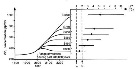
Uncertainty and Future Climate Policy

At present, it is not possible to uniquely relate greenhouse gas concentrations and temperature. The 2001 consensus among climate modelers was that a doubling of CO₂-equivalent concentrations would increase annual average global surface temperatures by 1.5-4.5^oC (IPCC, 2001a), though we noted in the section on climate sensitivity that this is an oversimplification and likely underestimates the range (see Climate Sensitivity).

Figure — Left: IPCC stabilization scenarios for atmospheric CO₂. Right: Corresponding equilibrium changes in global mean temperature since pre-industrial times (central values plus uncertainty ranges from IPCC (1996a). (Source: Azar & Rodhe, 1997.)

From this Figure, it can be seen that the global temperature increase for an atmospheric CO₂ concentration of 550ppm will only stay below 2^oC if the climate sensitivity is on the very low end of the IPCC's estimates.

Azar and Rodhe (1997) conclude that if climate sensitivity turns out to be in the upper range of the IPCC's estimates, then a CO₂ concentration of 550ppm will be sufficient to yield a global average temperature change of a magnitude approaching that which occurs over the thousands of years it takes to transition from an ice age to an interglacial period (roughly 5-7^oC). It appears that in order to have a very high probability of keeping the global temperature changes within the range of natural fluctuations that have occurred during the past few millennia (roughly 1^oC), the climate sensitivity has to be low or the atmospheric CO₂ concentration has to be stabilized at around 350ppm (i.e., below current levels).

The policy challenge that can be extracted from this is to ask whether 1) the burden of proof lies on those who argue that uncertainties which preclude confident prediction of the likelihood of exceeding any specific warming threshold — 2^oC for the IPCC stabilization scenarios — should lead to a “wait and see” policy approach, or, 2) if, rather, the burden of proof lies on those who, citing precautionary principles, believe it is not “safe” or acceptable to risk such potentially dangerous changes in the global climate system. However — and this is a primary message here — until it has been widely accepted with much higher confidence that a temperature increase above 2^oC is “safe” or that the climate sensitivity is lower than the central estimate, the projections shown in the IPCC stabilization scenarios suggest that the global climate policy community should not dismiss policies that lead to eventual stabilization in the range of 350-400 ppm.

When attempting to manage risk, a government should look at policy options that involve both adaptation and mitigation (Jones, 2003), though as stated by Perrings, 2003 and discussed earlier in this web site, many future climate risks, especially abrupt events, favor mitigation over adaptation. It is not suggested that governments adopt specific targets that should be strictly adhered to over the next hundred years. On the contrary, the UNFCCC recognizes that steps to understand and address climate change will be most effective “if they are continually reevaluated in the light of new findings in these areas” (UNFCCC, 1992). In IPCC language, “The challenge now is not to find the best policy today for the next hundred years, but to select a prudent strategy and to adjust it over time in the light of new information” (IPCC, 1996a). Christian Azar and I (Schneider and Azar, 2001) made a similar comment:

In our view, it is wise to keep many doors — analytically and from the policy perspective — open. This includes acting now so as to keep the possibility of meeting low stabilization targets open. As more is learned of costs and benefits in various numeraires and political preferences become well developed and expressed, interim targets and policies can always be revisited. But exactly how much near term abatement or other technology policies that are required to keep the option of low stabilization within reach is, of course, very difficult to answer, in particular because the inertia of the energy system, let al.one the political system, has proven difficult to model.

This revising of policy as new information becomes available is often referred to as Bayesian updating. Advocating the use of Bayesian updating in climate change policy has also been done by Perrings, 2003:

A crucial element of any precautionary approach is the mechanism by which the decision maker learns about the probability distribution of outcomes. Since uncertainty implies that there is scope for learning (although learning does not necessarily reduce uncertainty), every problem that is a candidate for a precautionary approach is also a candidate for learning. Precautionary action implies a mechanism for learning, or for updating the information on which decisions are taken since expectations about the payoff to different outcomes are conditional on the state of knowledge, and are therefore revised as the state of knowledge changes.

Governments will be better able to deal with this uncertainty if they promote research on all sides of the issue through research grants and endowments and encourage the foundation of climate-specific organizations like the California Climate Action Registry, which teaches companies to monitor their CO₂ emissions levels in an attempt to establish emissions baselines against which any future greenhouse gas reduction requirements may be applied; and the Green House Network, whose goal is to educate people everywhere about the need to stabilize the climate.

Research on sequential decision-making under uncertainty includes, e.g., Manne & Richels (1992), Kolstad (1994, 1996a, 1996b), Yohe and Wallace (1996), Lempert and Schlesinger (2000), Ha-Duong et al. (1997), Narain and Fisher (2003), Fisher (2001). The results of these studies are addressed in subsequent sections.

Go to top